Chapter 1 Fields – Basics

Aims of this section

At the end of this section you should be able to

Describe the concept of a field
State the link between potential and fields and calculate field strength from potentials.
Sketch electric field lines for distributions of charges.

1.1 What is a field?

Recommended reading: Tipler & Mosca 4.2, 21-4

A field is a region of space, where property of that space is characterized by either a number (a scalar field) or by three numbers (a vector field).

The concept of a field circumvents the problem of action at a distance where one inanimate object is “aware" that another has arrived.

Figure 1.1: Two objects ‘feeling’ each other’s prescence.

We understand that the first body sets up a field and the second body interacts with the first via this field. There is no need for action at a distance because the field of the 1st object is present in space whether or not the second object is there.

Figure 1.2: Two objects ‘feeling’ each other’s prescence with the help of a field.

1.1.1 Charges

Why does object 1 set up a field? Fields arise when objects have charge. Electric charges cause electromagnetic fields, but other fields arise from different types of charge for example gravitational fields arise from mass. (And the strong field that is responsible for holding quarks inside protons and neutrons arises from the colour charge – see Inside The Atom.)

There are two types of electric charge, \(+\) and \(-\). “Like" charges repel, while”unlike" charges attract. Electric charge is quantized: the elementary charge is \(1.6021773 \times 10^{-19}\) C and is the charge on the electron and the proton. Charges measured in laboratories are always multiples of this but the quarks inside protons and neutrons and other hadrons have charges that fractions of this elementary charge. Charge is conserved in all interactions we have observed. Most everyday objects are electrically neutral with the number of protons and electrons balanced, which hides the fact that they contain enormous amounts of \(+\) and \(-\) charge. Things that we would describe as “charged objects", have a small imbalance in charge.

Gravitational charge: there is one type of gravitational charge, which is mass/energy. Gravitational charges attract. We don’t know about quantization of mass. (You can probably spend many hours on the internet reading different opinions on this). Mass/Energy is conserved and all everyday objects are gravitationally charged so they all attract each other but gravity is very weak – we can easily pick up bits of paper with an electrically charged rod when rather few electrons have been moved.

Strong field charge: there are three types of fundamental strong charge (red, green and blue) + three anticharges. Charges attract. Colour is quantised and colour is conserved in interactions. All everyday objects are colour neutral. Colour fields are confined within subatomic particles i.e. to length scales of \(\sim 10^{-15}\) m.

1.2 Scalar and vector fields

A scalar field is characterized at each point by a single number. e.g. the temperature, \(T\), at each position in a block of metal heated at some places and cooled at others.

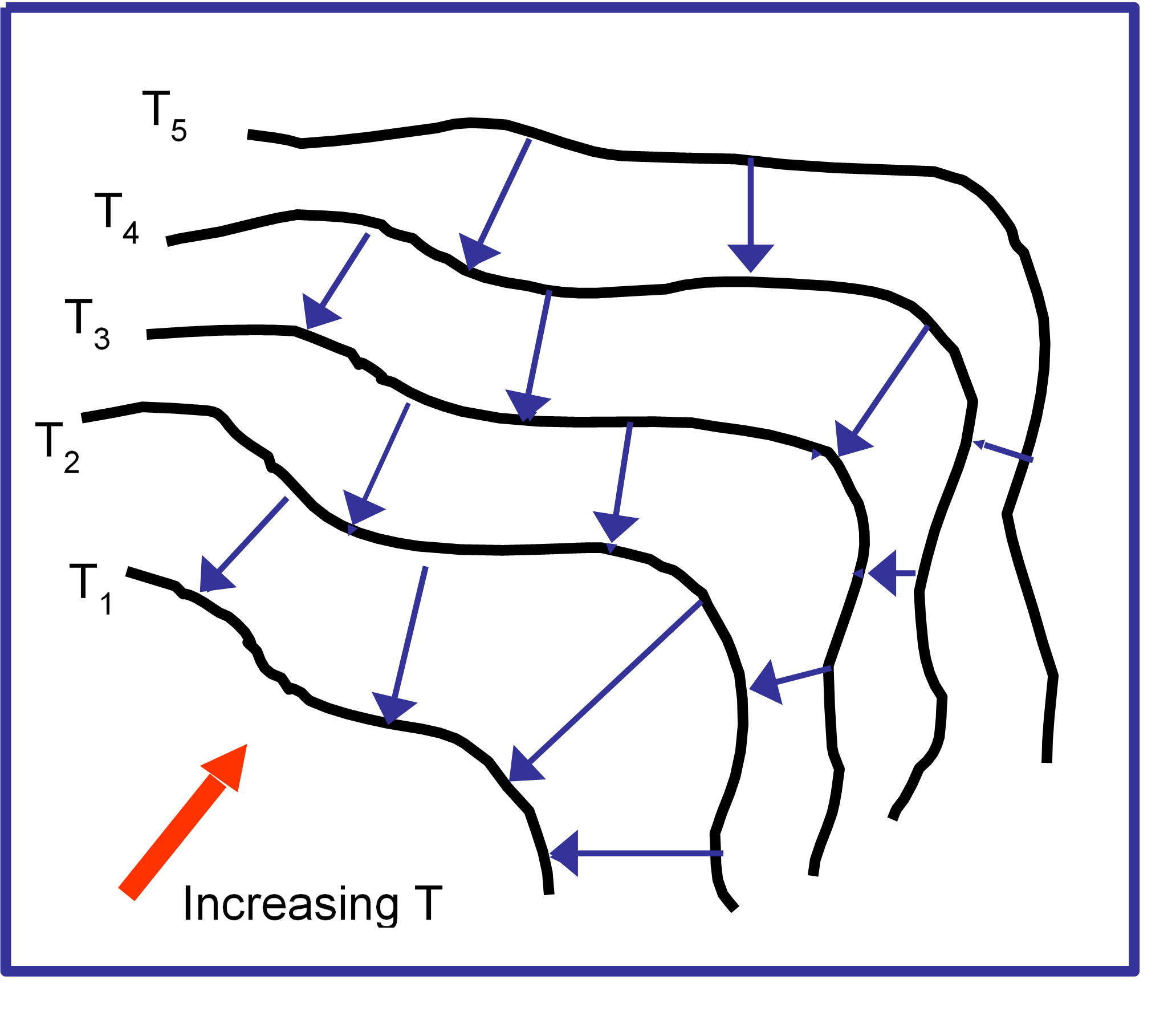
Contours of constant temperature i.e. isotherms. Temperature fields are scalar fields, having one value of temperature at each point in space. Heat flow, however, has an associated vector field, as it has a direction and magnitude for each point in space (blue arrows).

Figure 1.3: Contours of constant temperature i.e. isotherms. Temperature fields are scalar fields, having one value of temperature at each point in space. Heat flow, however, has an associated vector field, as it has a direction and magnitude for each point in space (blue arrows).

\(T\) is a function of position i.e. \(T = T(x,y,z)\). At every point we can measure the scalar value of the temperature \(T\). The black lines represent isotherms i.e. lines where the temperature is constant (\(T_1 < T_2 < T_3 < T_4 < T_5\)). Heat flow (blue arrows) is perpendicular to the contours of constant temperature - the isotherms (\(T_1\), \(T_2\) etc). The magnitude of the heat flow is proportional to the temperature gradient so that the heat flow is larger when isotherms are closer together.

The scalar temperature field has an associated vector field because at any point, the heat flow is a vector, the magnitude and direction of which depend on position. Heat flow is therefore a vector field which is related to the scalar field of temperature. The vector gradient of the field of heat flow depends on the temperature at each point.

1.3 Link between scalar and vector field

Recommended reading: Tipler & Mosca 23-3.

For the scalar temperature field \(T(x,y,z)\) the vector describing the direction and the magnitude of the maximum temperature gradient is:

\[\begin{equation} \tag{1.1} \text{Grad} \; T = \nabla T = \frac{\partial T} {\partial x} \hat{\mathbf{i}} + \frac{\partial T}{\partial y} \hat{\mathbf{j}} + \frac{\partial T}{\partial y} \hat{\mathbf{k}} \end{equation}\]

The heat flow is a vector given by \(\mathbf{Q} = -k \nabla T\); the minus sign is because heat flows from high temperature to low temperature.

In general, for a scalar potential \(-\nabla \phi = \frac{\partial \phi} {\partial x} \hat{\mathbf{i}} + \frac{\partial \phi}{\partial y} \hat{\mathbf{j}} + \frac{\partial \phi}{\partial y} \hat{\mathbf{k}}\) describes the magnitude and direction of the physical effects of the potential, with an appropriate constant if needed. In the case of the electric field if the electric potential is \(V\) then the vector field \(\mathbf{E} = -\nabla V\).

As an example, the gravitational field can be obtained from the gravitational potential. The scalar gravitational potential energy is given by \(U = mgz\) near the Earth’s surface, where \(z\) is the height. The gravitational potential is \(U/m = gz\). The gravitational field is \(-\nabla(gz)=-g \hat{\mathbf{k}}\).

1.3.1 Other operations on vectors

The vector operator \(\nabla\) behaves as a vector. We have looked at grad \(\nabla\phi\) where \(\phi\) is a scalar field. In Maxwell’s equations, which you cover next year, you will also meet \(\nabla\) operating on the electric field \(\mathbf{E}\):

\(\nabla \cdot \mathbf{E}\) (div or divergence)

\(\nabla \times \mathbf{E}\) (curl or rotation)

Maxwell’s equations are one of the great achievements of 19th century Physics. They link the phenomena of electricity and magnetism and can be used to derive an expression for the speed of light. Einstein said that the theory of Relativity was rooted in Maxwell’s equations. The equations in their differential form are shown below and we will meet most of the concepts in this course and integral versions of some of the laws. You can read more about Maxwell’s Equations in Chapter 30 of Tipler and Mosca.

\[\begin{equation} \tag{1.2} \nabla \cdot \mathbf{E} = \frac{\rho}{\epsilon_0} \end{equation}\]

\[\begin{equation} \tag{1.3} \nabla \times \mathbf{E} = - \frac{\partial \mathbf{B}}{\partial t} \end{equation}\]

\[\begin{equation} \tag{1.4} \nabla \cdot \mathbf{B} = 0 \end{equation}\]

\[\begin{equation} \tag{1.5} \nabla \times \mathbf{B} = \frac{\mathbf{j}}{c^2 \epsilon_0} + \frac{1}{c^2} \frac{\partial \mathbf{E}}{\partial t} \end{equation}\]

Source: http://www.clerkmaxwellfoundation.org/html/about_maxwell.html ; https://maxwells-equations.com/

1.4 Representing the electric field

Recommended reading: Tipler & Mosca 21-5.

The vector electric field, \(\mathbf{E}\), at a particular point in space, associated with a collection of charges, is defined in terms of the force, \(\mathbf{F}\), exerted on a positive test charge, \(q_0\), at that point \(E = F/q_0\).

\(\mathbf{E}\) has units of Vm\(^{-1}\) or NC\(^{-1}\). The electric field is normally represented by field lines that indicate what a positive test charge will do. The arrows indicate the direction of the field and the density of lines indicates the strength of the field at a point. The diagram shows the electric field lines for two positive point charges of the same magnitude.

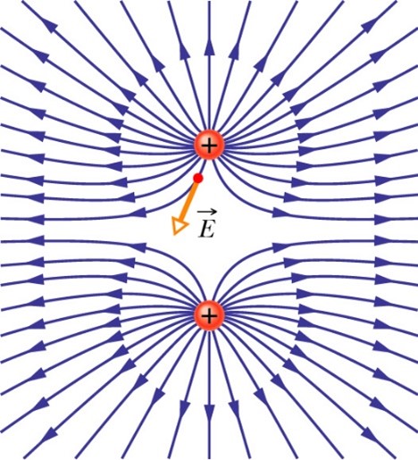
Figure 1.4: Representation of the electric field of two positive charges (like charges) placed close together.

Note that the field lines are symmetric as they leave the charges. They do not cross.

1.5 Equipotential surfaces

An equipotential surface is the surface of constant potential. The electric field is always perpendicular to the equipotential surface as the heat flow was always perpendicular to the isotherms in the temperature example. The picture shows an example of the equipotentials for a point charge. The field lines are in blue and the equipotentials the dashed black lines. The following website - http://www.falstad.com/emstatic/index.html - allows you to set up different charge configurations and see the field lines and equipotentials.

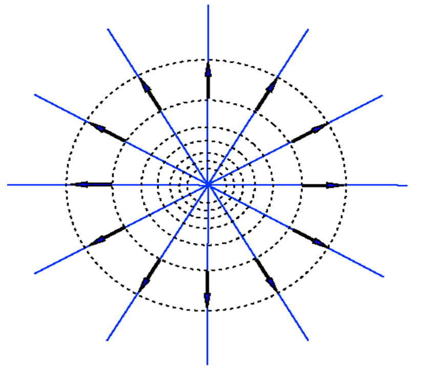
Representation of a field radiating outwards from a point (blue lines), showing how the equipotentials (black dotted lines) are always perpendicular to the field lines.

Figure 1.5: Representation of a field radiating outwards from a point (blue lines), showing how the equipotentials (black dotted lines) are always perpendicular to the field lines.

1.6 Summary

Fields arise from charges, and not just electric charges.
A scalar potential \(\Phi\) has an associated vector field \(-\nabla \Phi\) and the direction of the vector field is perpendicular to the equipotentials.
We represent fields with lines that show the direction of motion of a charge with the density of the field lines indicating the field strength.