Chapter 3 Magnetic Fields
3.1 The magnetic field
Recommended reading: Tipler & Mosca 26
In electrostatics, we viewed electric charges as interacting via the electric field to avoid action at a distance. The field surrounds any charge and when a second charge is brought near to the first it interacts with the field that is already present.
Can we think of “magnetic charges" interacting via the magnetic field, \(\mathbf{B}\)? No. This is because magnetic charges have not been found to exist - there is no evidence for single North or South poles. Searches have been made for magnetic monopoles, but without any success, although their existence has not been entirely ruled out. (This is way beyond our syllabus but if you are interested you could try looking at https://royalsocietypublishing.org/doi/10.1098/rsta.2018.0328.)
The magnetic field is produced by moving electric charges (i.e. electric currents). As with the electric field, the magnetic field can be represented using field lines and the density of field lines represents the strength of the field and the direction is that in which a north pole would move.
The magnetic field \(\mathbf{B}\) is measured in the SI unit of Tesla or in Gauss: 1 Tesla = \(10^4\) Gauss = \(\frac{\mathrm{Ns}}{\mathrm{Cm}} = \frac{\mathrm{N}}{\mathrm{Am}}\).
There are some important differences between the behaviour of charges in electric and magnetic fields. In electric fields, the force on a charge is parallel to the field lines – a positive charge moves along the field lines in the direction indicated. In magnetic fields, the force on a moving charge is perpendicular to the field lines.
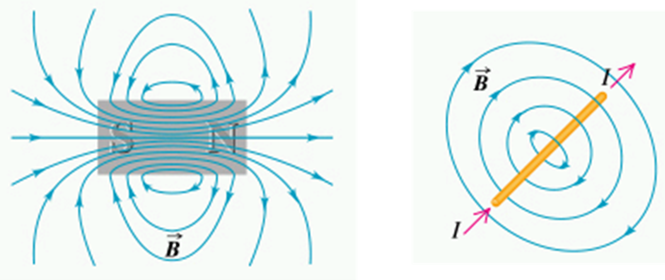
Figure 3.1: Left: The magnetic field produced by a bar magnet. Right: Section of a wire (yellow) carrying current I and the magnetic field B that it produces.
Magnetic field lines always form closed loops whereas electric field lines begin and end on charges. This means that a version of Gauss’ Law for magnetism states \(\Phi_B =\) ∯ \(\mathbf{B} \cdot \mathrm{d} \mathbf{S} = 0\) (see Tipler & Mosca, 27-3). As field lines are closed all field lines entering a closed surface must leave it as well. So net magnetic flux through the surface is zero.
The direction of the magnetic field direction due to an electric current is given by the right-hand rule. If you point the thumb of your right hand in the direction of the current and then curl the fingers the field is in the direction of the curl of your fingers.
3.2 Forces from Magnetic Fields
Recommended reading: Tipler & Mosca 26-2
The Lorentz force describes the force felt by a moving charge in a combination of electric and magnetic fields.
\[\begin{equation} \tag{3.1} \mathbf{F} = q(\mathbf{E} + \mathbf{v} \times \mathbf{B}) \end{equation}\]
The cross product tells us that force due to the magnetic field \(\mathbf{B}\) is perpendicular to the magnetic field and the velocity of a charged particle (\(\mathbf{v}\)) and therefore when the velocity and magnetic field are parallel (or antiparallel) to each other, the force on the charged particle due to the magnetic field is zero. Since the magnetic force, is always perpendicular to the velocity vector of the particle it cannot do any work on the charge and therefore cannot change the energy and speed of the particle.
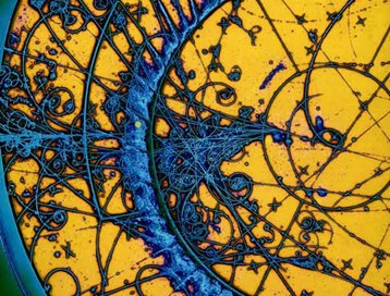
Figure 3.2: Enhanced image of the traces in a bubble chamber, which shows the paths of charged particles.
The artistically enhanced image above was produced by the Big European Bubble Chamber (BEBC), which started up at CERN in 1973. Charged particles passing through a chamber filled with hydrogen-neon liquid leave bubbles along their paths (Image: BEBC). You can see the spiral paths of the charged particles as they move in circles under the influence of the magnetic field but lose energy through collisions with the Hydrogen-neon atoms.
3.2.1 JJ Thomson’s measurement of \(e/m\)
As seen in the previous exercise, the electric and magnetic forces on a charged particle are equal if \(E = vB\), i.e. when the speed of the particle is given by \(E/B\). This condition doesn’t depend on the mass or the charge of the object. JJ Thomson used this to make a measurement of \(e/m\) for the “cathode rays" demonstrating that these rays consisted of particles. The principle of the experiment is to apply crossed electric and magnetic fields, that is electric and magnetic fields at right angles to each other. First the deflection in the \(E\) field only is measured. In this case the force depends on charge and the deflection on mass and \(v\). A magnetic field is that applied to give an overall deflection of zero. At this point the forces due to \(\mathbf{E}\) and \(\mathbf{B}\) are balanced and the velocity of the particle is therefore measured and can be used with the 1st result, for the \(E\) field only, to calculate the charge/mass ratio.
3.2.2 Circulating charges
Recommended reading: Tipler & Mosca 26-2
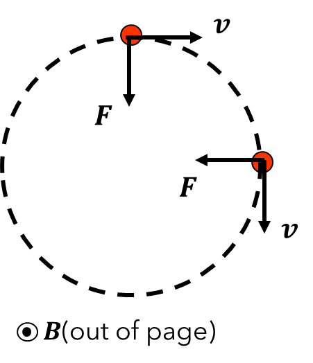
Figure 3.3: A charged particle travelling with velocity $ $ along a circular path in a magnetic field B. The magnetic field provides the centripetal force F causing the circular motion.
If \(\mathbf{B}\) and \(\mathbf{v}\) are perpendicular, a particle moving in a constant \(\mathbf{B}\) field is forced to move in a circle by the (centripetal) magnetic force. Note that if there is a component of \(v\) in the same direction as \(\mathbf{B}\) there is no force in this direction and that component of the velocity is unchanged in direction or magnitude causing the particle to move in a spiral. The frequency of rotation around the circle is the cyclotron frequency. This frequency does not depend on the particle velocity or the radius of the circle.
Charged particles will tend to spiral along field lines. By shaping the magnetic field lines as shown in , it is possible to confine charged particles inside a “magnetic bottle".
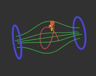
Figure 3.4: A magnetic bottle: Magnetic field shape (green lines) that allows a moving charged particle to be confined within the field lines. Search ‘magnetic bottle’ on YouTube to see a demonstration of how this works.
Charged particles are also confined along the Earth’s field lines. This protects us from cosmic radiation and is also responsible for the northern and southern lights.
3.2.3 Magnetic force on a wire
We can use the expression for the force on a single charge due to a magnetic field to calculate the force on a length of wire carrying a current. This arguments is describe below but you can also look at the derivation in Tipler & Mosca (26-1).
The expression for the force on a moving charge in a current carrying conductor in a magnetic field is \(\mathbf{F} = q\mathbf{v}_d \times \mathbf{B}\) (where \(\mathbf{v}_d\) is the drift velocity for the charge carriers). The current is the rate at which charge passes any point on the wire and this is just \(nqv_d\) where \(n\) is the number of charge carriers per unit length. Note that if the carriers are positive then the vector \(qv_d\) points in the direction of conventional current flow. If \(q\) is negative \(v_d\) points in a direction opposite to conventional current flow but the combination \(qv_d\) points in the direction of conventional current flow. The force per unit length on the wire is \(nq \mathbf{v}_d \times \mathbf{B}\) and the force on a length \(L\) of wire is \(Lnq \mathbf{v}_d \times \mathbf{B}\). We define \(\mathrm{L}\) as the vector length of the wire i.e. a vector with length equal to the length of the wire and in the direction of the flow of conventional current. \(\mathrm{L}\) therefore points in the direction of \(q \mathbf{v}_d\) so \(\mathrm{L} \times \mathbf{B}\) is in the direction of the force on the wire and, since \(I = nq v_d\), the force is given by \(\mathbf{F} = I \mathrm{L} \times \mathbf{B}\).
3.2.4 Force on current loops & motors
Recommended reading: Tipler & Mosca 26-3
The force on a current carrying conductor in a magnetic field \(\mathbf{F} = I \mathrm{L} \times \mathbf{B}\) can be used to make a motor. The principle of operation of a motor made of a single loop of wire is shown nicely in http://www.walter-fendt.de/html5/phen/electricmotor_en.htm.
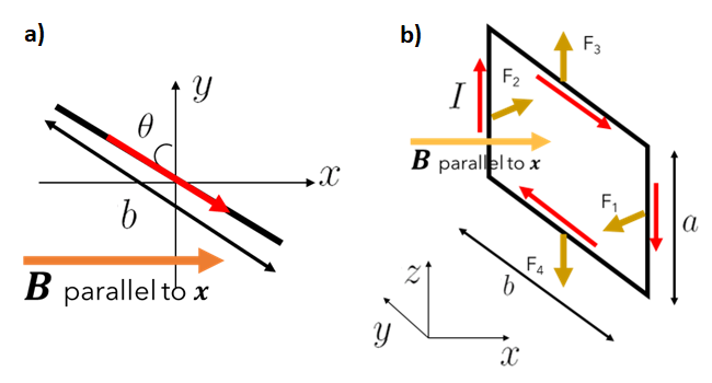
Figure 3.5: extbf{a)} The top of a wire loop as viewed from the positive z-direction. The red arrow shows the direction of the current I. The loop is subject to magnetic field B in a direction parallel to the x-axis. extbf{b)} Side view of the same current loop as in extbf{a)}, showing the direction of the forces on each of the four sides of the loop - F_1, F_2, F_3 and F_4.
The length of the coil as viewed in a) above is \(b\). The current at the top of the loop as viewed from positive \(z\) is flowing down the page to the right. Using the right-hand rule to work out the direction of \(\mathrm{L} \times \mathbf{B}\) gives a force in the positive \(z\)-direction. This will be balanced by the force from the other end of the loop (where the current flows in the opposite direction. These sides do not produce a torque. In a), the sides of length \(a\) are directed into the page. At the lower end of a), the current flows into the page in the negative \(z\)-direction so \(\mathrm{L}\) is in the negative \(z\)-direction and the field \(\mathbf{B}\) is in the positive \(x\)-direction. Since \(-\hat{\mathbf{k}} \times \hat{\mathbf{i}} = \hat{\mathbf{i}}\), the force on that side is therefore in the negative \(y\)-direction. On the other side of the loop the current is reversed but not the field so that the force is in the opposite direction. The magnitude of the force is the length of the side, \(a\), multiplied by the current and the magnitude of the magnetic field. To calculate the torque now needs the perpendicular distance from the point the force acts to the centre of the loop: this is \(\frac{b}{2}\sin\theta\). The torque about the \(z\)-axis due to one side of the loop is \(\frac{BIab}{2} \sin \theta\). Since there are two sides contributing to the torque the final answer is \(\Gamma = BIab \sin\theta\). Note that this depends on the area of the loop, \(ab\).
3.2.5 Torque on a coil
For a single loop the torque is \(\Gamma = BIab \sin\theta\), noting that \(ab\) is the area of the loop. If instead of a single loop there is a coil with \(N\) loops then the torque is simply multiplied by \(N\), hence \(\Gamma = NBIab \sin\theta\). By analogy with the electric dipole, we can define a magnetic dipole moment \(\boldsymbol{\mu} = IA \hat{\mathbf{n}}\), where \(\hat{\mathbf{n}}\) is a unit vector in the direction normal to the area \(A\). So we can express the torque as \(\Gamma = \boldsymbol{\mu} \times \mathbf{B}\).
3.3 The Biot-Savart Law
Recommended reading: Tipler & Mosca 27-1, 27-2
We can generalize our previous result for the force on a current \(F = IL \times B\) by considering a small element of current \(dF = I \mathrm{d} s \times B\) and then calculate the field due to a sum of current elements where these do not necessarily lie on a straight line or other simple shape. The magnetic field could have been produced by another current which give us interactions between currents.
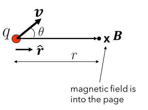
Figure 3.6: A point charge q moving with velocity v produces a magnetic field B at point x, which is a distance r from the charge.
A point charge, \(q\) ,moving with velocity, \(v\), produces a magnetic field \(B\) at a distance \(r\) in a direction given by \(\mathbf{v} \times \hat{\mathbf{r}}\), where \(\hat{\mathbf{r}}\) points from \(q\) to the point where the field is measured.
\[\begin{equation} \tag{3.2} \mathbf{B} = \frac{\mu_0}{4\pi} q \mathbf{v} \times \frac{\hat{\mathbf{r}}}{r^2} \end{equation}\]
The magnetic field at point \(P\) due to the current element \(I \mathrm{d}\mathbf{s}\) is therefore
\[\begin{equation} \tag{3.3} \mathrm{d} \mathbf{B} = \frac{\mu_0}{4\pi} I \mathrm{d}\mathbf{s} \times \mathbf{r} /r^2 \end{equation}\]
or, in terms of the magnitudes, \[\begin{equation} \tag{3.4} \mathrm{d} B = \frac{\mu_0}{4\pi} \frac{I \mathrm{d} s \sin\theta}{r^2} \end{equation}\]
This is the Biot-Savart Law, which is analogous to Coulomb’s Law for evaluating the electric field due to a point charge. The Biot-Savart Law can be used to calculate the field due to a set of conductors.
3.4 Ampère’s Law
Recommended reading: Tipler & Mosca 27-4
Ampère’s Law states that the sum (or integral) of the product \(\mathbf{B} \cdot \mathrm{d}\mathbf{s}\) around a closed loop is equal to the total current flowing through the surface enclosed by the loop multiplied by the permeability of free space, \(\mu_0\). Mathematically,
\[\begin{equation} \tag{3.5} \oint \mathbf{B} \cdot \mathrm{d} \mathbf{s} = \mu_0 I \end{equation}\]
where \(\mathrm{d}\mathbf{s}\) is a vector that points along the tangent to the loop with a magnitude equal to a small length of the curve.
To use Ampère’s law we construct an imaginary Ampèrian loop around some current carrying conductors. (Compare this to constructing a Gaussian surface around charges to determine the electric flux and hence the field.) In this case the loop is arranged so it is parallel to or perpendicular to the magnetic field so \(\mathbf{B} \cdot \mathrm{d}\mathbf{s} =|\mathbf{B}||\mathrm{d}\mathbf{s}|\) or \(\mathbf{B}\cdot \mathrm{d}\mathbf{s} = 0\) respectively.
We will solve symmetric problems in this way as there are limitations to Ampère’s law (discussed in Tipler & Mosca 27-4). We evaluate the line integral of \(\mathbf{B}\) around the loop which is equal to the sum of the current flowing through the loop. (Compare with Gauss’s Law where the integral of \(\mathbf{E}\) over a surface was equal to the charge enclosed by the surface.)
We’ll consider a couple of classic examples of using Ampère’s Law:
A single wire carrying current
The magnetic field of a solenoid
3.4.1 Example: Magnetic field of a wire
Consider the field outside a single wire carrying current and determine the field at a distance \(R\) from the wire. From the symmetry of the problem the field lines are circular about the wire and the field has a constant magnitude at a constant distance from the wire. So we pick a loop that is also circular. The magnitude of \(\mathbf{B}\) is constant along the loop and the loop is always parallel to \(\mathbf{B}\).
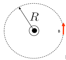
Figure 3.7: Top view of a wire carrying current out of the page. The magnetic field lines form loops (dotted line) in the direction shown by the red arrow. The magnetic field strength at a distance R from the wire can be found using Ampere’s Law.
Ampère’s Law states \(\oint \mathbf{B} \cdot \mathrm{d}\mathbf{s} = \mu_0 I\). If we perform the integral in the clockwise direction then the element of the path \(\mathrm{d}\mathbf{s}\) is parallel to B and so the integral is the magnitude of B multiplied by the magnitude of ds integrated around the path. This is simply the length of the path times the magnitude of \(\mathbf{B}\):
\[\begin{equation} \tag{3.6} \oint \mathbf{B} \cdot \mathrm{d}\mathbf{s} = B \times 2\pi r = \mu_0 I \end{equation}\]
Rearranging gives
\[\begin{equation} \tag{3.7} B = \frac{\mu_0 I}{2\pi R} \end{equation}\]
as for Biot-Savart Law – as we would expect.
3.4.2 Example: Magnetic field of a solenoid
A solenoid is a wire wound in a long straight helix with the length usually much longer than the diameter. It looks like a set of coils next to each other and the overall field is the same as a for a bar magnet of the same shape.
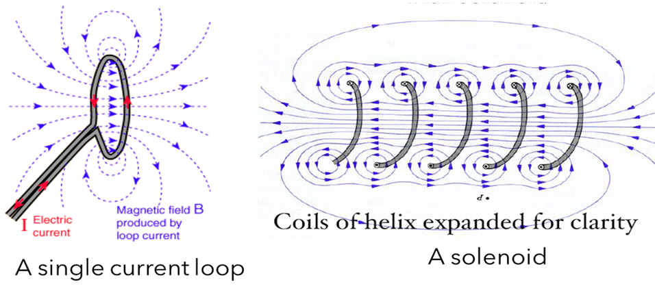
Figure 3.8: Representation of the magnetic field lines produced by: a single current loop (left); and a solenoid (right).
In this example we calculate the magnetic field of a long solenoid with \(n\) turns per unit length. As the length tends to infinity, the field outside tends to zero and the field inside becomes increasingly uniform and parallel to the axis. We need to find a suitable Ampèrian loop (see figure below). In this case we pick a rectangular loop where one side (a-b) lies within the solenoid and is parallel to the field. One side (c-d) is outside the solenoid where the field is 0. And the two remaining sides are partly perpendicular to the field and partly in a field free region.
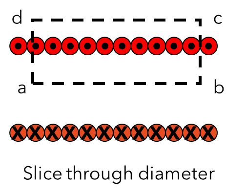
Figure 3.9: Cross-section of a solenoid, taken through the diameter of the loops. Hence the top row of wires carry current coming out of the page and the bottom row of wires carry current into the page.
The only contribution to \(\oint \mathbf{B} \cdot \mathrm{d}\mathbf{s}\) from the loop is the side ab where, in this case, the field is parallel to the path. Since \(\mathbf{B}\) is uniform along the path \(\oint \mathbf{B} \cdot \mathrm{d}\mathbf{s} = BL\) where \(L\) is the length of the path from a to b.
The total current enclosed by the loop is the number of turns per unit length in the solenoid multiplied by the current, \(nIL\). \[\begin{equation} \tag{3.8} \therefore \oint \mathbf{B} \cdot \mathrm{d}\mathbf{s} = BL = \mu_0 nIL \\ \therefore B = \mu_0 nI \end{equation}\]
3.5 Faraday’s Law of induction
A changing magnetic flux in a circuit will produce a current that opposes that change. Faraday’s Law of induction relates the induced EMF in a circuit to the rate of change of magnetic flux through a circuit.
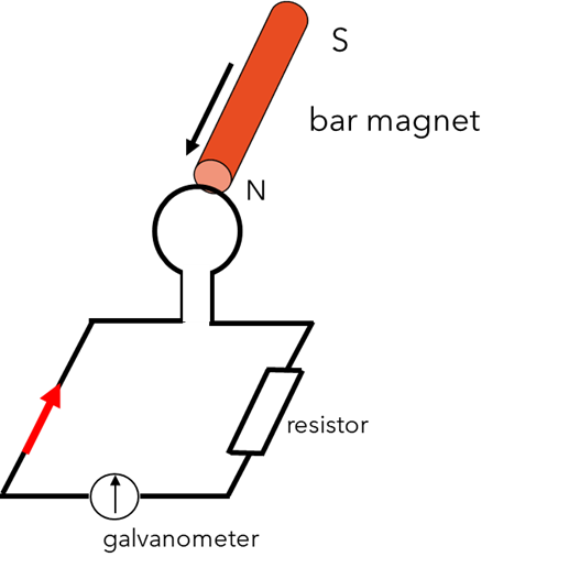
Figure 3.10: Current loop including a resistor and a galvanometer. The red arrow indicates the direction of the current. A bar magnet is moved towards and away from the coil.
Consider the case of the circuit shown in that has a loop of wire.
If the magnet is stationary: no current flows
If the magnet moves towards the coil : current flows while the motion continues.
If the magnet moves away from the coil : the current flows in opposite direction
If a north pole is replaced by a south pole, then the current flow reverses in direction.
If the magnet moves faster the current is increased.
The induced current is a result of an induced electromotive force (emf), which depends on the rate of change of magnetic flux through the loop. We have already discussed electric flux in Gauss’ Law and we’re using the same idea here for Faraday’s Law of induction. The changing flux through the circuit could be due to a magnetic field produced by a second circuit.
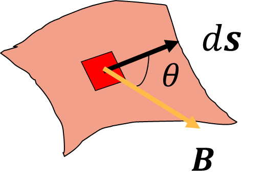
Figure 3.11: A magnetic field B passing through an arbitrarily-shaped surface. The vector ds is the infinitesimal vector perpendicular to the surface. θ is the angle between ds and the direction of the magnetic field.
The magnetic flux through a surface is the component of the field perpendicular to the surface multiplied by the area of the surface. Mathematically
\[\begin{equation} \tag{3.9} \Phi_B = \int\mathbf{B} \cdot \mathrm{d}\mathbf{s} \\ \text{or} \; \Phi_B = \int \mathbf{B} \cos\theta \mathrm{d} s \end{equation}\]
where, as with Gauss’s Law, \(\mathrm{d} \mathbf{s}\) is a vector perpendicular to the surface and with magnitude equal to the area of an element of the surface. We take the dot product to extract the component of \(\mathbf{B}\) perpendicular to the surface. Magnetic flux is measured in Webers (Wb). You can see that this must be equivalent to T m\(^2\) and, less obviously, Vs.
Faraday’s Law states that the induced emf in a circuit is equal to the negative of the rate of change of flux through the circuit, written as
\[\begin{equation} \tag{3.10} V = - \frac{\mathrm{d} \Phi_B}{\mathrm{d} t} \end{equation}\]
If rather than a single loop of wire a coil has \(N\) turns close together then the induced emf is simply multiplied by \(N\).
3.5.1 Transformers
There are a number of devices that use inductance to useful effect. Transformers are one such device.
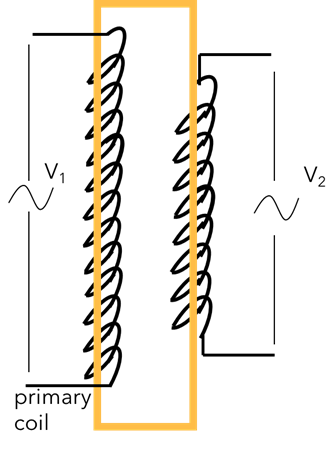
Figure 3.12: Schematic of a transformer. A voltage V_1 is applied to the primary coil (left), which induces a different voltage V_2 in the secondary coil (right).
Transformers (see ) consist of two or more coils (usually with a ferromagnetic core) so that the field from one coil is coupled to the other coil. An AC voltage applied to the primary coil (\(V_1\)) is transformed to a different voltage at the secondary coil (\(V_2\)).
\[\begin{equation} \tag{3.11} \frac{V_2}{V_1} = \frac{N_2}{N_1} \end{equation}\]
where \(N_1\) and \(N_2\) are the number of turns in the primary and secondary coils, respectively.
If \(N_2 > N_1\), then the output voltage from the secondary coil can be much larger than the voltage in the primary coil and this can be used to produce very high voltages for example, for an extra high tension (EHT) supply. If \(N_2 < N_1\), then the output voltage from the secondary coil is smaller but the output current can be very large for use in high current applications such as welding power supplies.
3.5.2 Dynamo
A dynamo is a type of generator, where a generator refers to a device that turns mechanical motion into electrical energy.
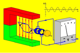
Figure 3.13: Schematic diagram of a dynamo, a type of generator, where the rotation of a coil generates an alternating current.
is taken from http://www.walter-fendt.de/html5/phen/generator_en.htm, an app which allows you to simulate a generator by changing certain parameters.
The dynamo functions as the opposite of a motor. In a motor a current applied to a coil in a magnetic field generates kinetic energy. In a dynamo the rotation of a coil in a magnetic field generates an alternating current.
3.5.3 The moving coil microphone
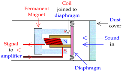
Figure 3.14: Schematic diagram of a moving coil microphone. Inside the microphone there is a diaphragm which is free to move. The diaphragm is attached to a coil, which is placed in the magnetic field of a permanent magnet.
In a moving coil microphone, movement of the diaphragm by sound entering the device cause the coil to move in the field of the magnet generating a varying current that can be amplified.
3.6 Lenz’s Law
Recommended reading: Tipler & Mosca 28-3
Lenz’s Law states that the induced emf and induced current are in such a direction as to oppose the change that induces them.
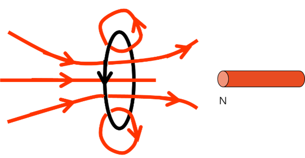
Figure 3.15: A current loop and its associated magnetic field (left) and a bar magnet (right).
Consider the bar magnet and current loop in . The motion of the N pole towards the loop induces a current which flows so as to induce a N pole closest to the magnet’s N pole, and hence repel it.
Lenz’s Law can be used to work out the direction of the induced current (or the sign of the induced emf if the loop is not closed).
Note that the agent causing the motion, in this case the magnet, experiences a resisting force and so work is done. This work is equal to the internal energy produced in the coil by the current flow.
(It is interesting to consider what would happen if instead of opposing the motion, the resulting current actually assisted it. In that case the motion of a N pole towards a loop would induce a S pole in the loop. This S pole would attract the N pole producing an acceleration that would in turn produce a larger current and hence a larger attraction etc. etc. This would violate the Principle of Conservation of Energy.
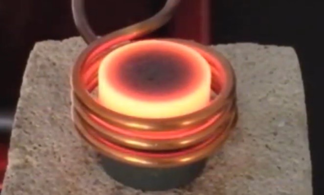
In short, Lenz’s Law is associated with opposing change. Another way of interpreting it is to consider that the current will flow in such a way as to oppose the change in magnetic field through the loop. When the magnetic flux through a large conductor changes, eddy currents are induced. These currents produce the heating shown in the inductive heater at the end of .
3.7 Inductance
Recommended reading: Tipler & Mosca 28-6
We have considered the case of an emf induced in a loop by a changing flux resulting from a changing current in another loop. However, such an emf can be induced by a changing flux through a coil brought about by a changing current in the same coil. This is known as the self-inductance, or more commonly just the inductance of the coil, and is usually represented by the symbol \(L\). The SI unit of inductance is the Henry, equivalent to kg m\(^2\) s\(^{-2}\) A\(^{-2}\).
The inductance relates the induced emf to the rate of change of current for a particular coil. So the voltage across an ideal inductor is given by \(V = -L \frac{\mathrm{d} I}{\mathrm{d} t}\). An ideal inductor has zero resistance, and we would treat a real inductor as a combination of a resistor and inductor in series.
The inductance of a solenoid is given by \[L = \frac{\mu_0 n^2 A}{l}\]
Note that this result depends only on the geometry of the coil and not on the voltage or the current. If the coil is filled with a magnetic material such as iron, the inductance, can be increased by a factor of \(10^3\) – \(10^4\).
In the next section of this course, we’ll look at electrical circuits that include resistance, capacitance and inductance and in particular at their response to alternating voltages.